How To Use A Dso For Car Repair

Instrument for displaying time-varying signals

A Tektronix model 475A portable analog oscilloscope, a typical instrument of the tardily 1970s

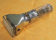
Oscilloscope cathode-ray tube

An oscilloscope, previously chosen an oscillograph,^[ane] ^[2] and informally known as a scope or o-scope, CRO (for cathode-ray oscilloscope), or DSO (for the more modern digital storage oscilloscope), is a blazon of electronic test instrument that graphically displays varying signal voltages, ordinarily as a calibrated ii-dimensional plot of one or more than signals as a office of fourth dimension. The displayed waveform can and then be analyzed for properties such every bit aamplitude, frequency, rising time, time interval, baloney, and others. Originally, calculation of these values required manually measuring the waveform confronting the scales built into the screen of the instrument.^[3] Modern digital instruments may summate and brandish these properties directly.

The oscilloscope tin can exist adjusted so that repetitive signals can be displayed as persistent waveforms on the screen. A storage oscilloscope can capture a single event and display it continuously, so the user can observe events that would otherwise appear too briefly to exist seen direct.

Oscilloscopes are used in the sciences, medicine, technology, automotive and the telecommunications industry. General-purpose instruments are used for maintenance of electronic equipment and laboratory piece of work. Special-purpose oscilloscopes may exist used to analyze an automotive ignition system or to brandish the waveform of the heartbeat as an electrocardiogram, for case.

Early on oscilloscopes used cathode ray tubes (CRTs) as their brandish element (hence they were often referred to every bit CROs) and linear amplifiers for signal processing. Storage oscilloscopes used special storage CRTs to maintain a steady brandish of a single brief signal. CROs were afterward largely superseded by digital storage oscilloscopes (DSOs) with sparse panel displays, fast analog-to-digital converters and digital bespeak processors. DSOs without integrated displays (sometimes known as digitisers) are available at lower cost and use a general-purpose computer to process and brandish waveforms.

History [edit]

This section needs expansion. You lot tin can assistance by adding to it. (June 2021)

The Braun tube was known in 1897, and in 1899 Jonathan Zenneck equipped information technology with axle-forming plates and a magnetic field for sweeping the trace.^[4] Early cathode ray tubes had been applied experimentally to laboratory measurements as early as the 1920s, only suffered from poor stability of the vacuum and the cathode emitters. V. Thousand. Zworykin described a permanently sealed, high-vacuum cathode ray tube with a thermionic emitter in 1931. This stable and reproducible component immune General Radio to manufacture an oscilloscope that was usable outside a laboratory setting.^[three] Later on World War II surplus electronic parts became the ground for the revival of Heathkit Corporation, and a $l oscilloscope kit made from such parts proved its premiere marketplace success.

Features and uses [edit]

oscilloscope showing a trace with standard inputs and controls

An analog oscilloscope is typically divided into four sections: the display, vertical controls, horizontal controls and trigger controls. The display is usually a CRT with horizontal and vertical reference lines called the graticule. CRT displays also have controls for focus, intensity, and beam finder.

The vertical department controls the amplitude of the displayed point. This section has a volts-per-segmentation (Volts/Div) selector knob, an AC/DC/Ground selector switch, and the vertical (principal) input for the instrument. Additionally, this section is typically equipped with the vertical beam position knob.

The horizontal section controls the fourth dimension base or "sweep" of the instrument. The primary command is the Seconds-per-Division (Sec/Div) selector switch. As well included is a horizontal input for plotting dual 10-Y centrality signals. The horizontal axle position knob is generally located in this department.

The trigger department controls the start event of the sweep. The trigger tin be set to automatically restart after each sweep, or tin exist configured to respond to an internal or external event. The primary controls of this department are the source and coupling selector switches, and an external trigger input (EXT Input) and level adjustment.

In addition to the bones instrument, most oscilloscopes are supplied with a probe. The probe connects to any input on the instrument and typically has a resistor of ten times the oscilloscope's input impedance. This results in a .1 (‑10X) attenuation gene; this helps to isolate the capacitive load presented by the probe cablevision from the betoken being measured. Some probes have a switch assuasive the operator to bypass the resistor when appropriate.^[3]

Size and portability [edit]

Nearly modern oscilloscopes are lightweight, portable instruments compact enough for a single person to deport. In improver to portable units, the market offers a number of miniature battery-powered instruments for field service applications. Laboratory grade oscilloscopes, especially older units that use vacuum tubes, are generally bench-top devices or are mounted on dedicated carts. Special-purpose oscilloscopes may exist rack-mounted or permanently mounted into a custom instrument housing.

Inputs [edit]

The signal to be measured is fed to ane of the input connectors, which is usually a coaxial connector such every bit a BNC or UHF type. Bounden posts or banana plugs may be used for lower frequencies. If the signal source has its ain coaxial connector, then a simple coaxial cable is used; otherwise, a specialized cable chosen a "telescopic probe", supplied with the oscilloscope, is used. In full general, for routine utilise, an open wire test atomic number 82 for connecting to the bespeak being observed is not satisfactory, and a probe is generally necessary. Full general-purpose oscilloscopes usually present an input impedance of one megohm in parallel with a small but known capacitance such as xx picofarads.^[5] This allows the employ of standard oscilloscope probes.^[six] Scopes for use with very high frequencies may have 50‑ohm inputs. These must be either connected directly to a 50‑ohm signal source or used with Z₀ or active probes.

Less-frequently-used inputs include i (or two) for triggering the sweep, horizontal deflection for X‑Y fashion displays, and trace brightening/concealment, sometimes called z'‑axis inputs.

Probes [edit]

Open wire examination leads (flight leads) are likely to choice up interference, and then they are non suitable for depression level signals. Furthermore, the leads have a high inductance, then they are not suitable for high frequencies. Using a shielded cablevision (i.east., coaxial cable) is amend for low level signals. Coaxial cable also has lower inductance, merely it has higher capacitance: a typical l ohm cable has most 90 pF per meter. Consequently, a one-meter directly (1X) coaxial probe loads a circuit with a capacitance of about 110 pF and a resistance of one megohm.

To minimize loading, attenuator probes (east.yard., 10X probes) are used. A typical probe uses a 9 megohm series resistor shunted by a low-value capacitor to make an RC compensated divider with the cable capacitance and telescopic input. The RC fourth dimension constants are adapted to match. For example, the 9 megohm series resistor is shunted by a 12.ii pF capacitor for a time abiding of 110 microseconds. The cable capacitance of 90 pF in parallel with the scope input of twenty pF and ane megohm (total capacitance 110 pF) also gives a time constant of 110 microseconds. In exercise, at that place is an aligning so the operator can precisely match the low frequency time constant (called compensating the probe). Matching the time constants makes the attenuation independent of frequency. At low frequencies (where the resistance of R is much less than the reactance of C), the excursion looks like a resistive divider; at high frequencies (resistance much greater than reactance), the circuit looks similar a capacitive divider.^[seven]

The result is a frequency compensated probe for pocket-size frequencies. It presents a load of about x megohms shunted past 12 pF. Such a probe is an comeback, simply does non piece of work well when the time scale shrinks to several cablevision transit times or less (transit time is typically 5 ns).^{[ description needed ]} In that time frame, the cablevision looks like its characteristic impedance, and reflections from the transmission line mismatch at the scope input and the probe causes ringing.^[viii] The mod scope probe uses lossy low capacitance manual lines and sophisticated frequency shaping networks to make the 10X probe perform well at several hundred megahertz. Consequently, there are other adjustments for completing the compensation.^[ix] ^[10]

Probes with 10:one attenuation are by far the virtually common; for big signals (and slightly-less capacitive loading), 100:ane probes may exist used. There are also probes that contain switches to select 10:1 or direct (1:1) ratios, but the latter setting has pregnant capacitance (tens of pF) at the probe tip, considering the whole cablevision'southward capacitance is and so directly connected.

Most oscilloscopes provide for probe attenuation factors, displaying the effective sensitivity at the probe tip. Historically, some motorcar-sensing circuitry used indicator lamps behind translucent windows in the panel to illuminate dissimilar parts of the sensitivity calibration. To do so, the probe connectors (modified BNCs) had an extra contact to define the probe'southward attenuation. (A sure value of resistor, connected to ground, "encodes" the attenuation.) Because probes article of clothing out, and because the automobile-sensing circuitry is not uniform between different oscilloscope makes, automobile-sensing probe scaling is not foolproof. Likewise, manually setting the probe attenuation is prone to user fault. Setting the probe scaling incorrectly is a common error, and throws the reading off by a gene of 10.

Special high voltage probes class compensated attenuators with the oscilloscope input. These have a large probe trunk, and some require partly filling a canister surrounding the serial resistor with volatile liquid fluorocarbon to displace air. The oscilloscope end has a box with several waveform-trimming adjustments. For safety, a bulwark disc keeps the user's fingers away from the signal being examined. Maximum voltage is in the low tens of kV. (Observing a high voltage ramp can create a staircase waveform with steps at dissimilar points every repetition, until the probe tip is in contact. Until and so, a tiny arc charges the probe tip, and its capacitance holds the voltage (open excursion). As the voltage continues to climb, another tiny arc charges the tip farther.)

There are also current probes, with cores that surroundings the usher carrying electric current to be examined. 1 type has a hole for the conductor, and requires that the wire be passed through the pigsty for semi-permanent or permanent mounting. Still, other types, used for temporary testing, have a two-office core that can be clamped around a wire. Inside the probe, a coil wound around the core provides a current into an appropriate load, and the voltage across that load is proportional to current. This blazon of probe but senses Air-conditioning.

A more-sophisticated probe includes a magnetic flux sensor (Hall effect sensor) in the magnetic circuit. The probe connects to an amplifier, which feeds (low frequency) current into the ringlet to cancel the sensed field; the magnitude of the current provides the low-frequency part of the current waveform, right downwards to DC. The curlicue still picks upwards loftier frequencies. In that location is a combining network akin to a loudspeaker crossover.

Front panel controls [edit]

Focus command [edit]

This control adjusts CRT focus to obtain the sharpest, virtually-detailed trace. In do, focus must exist adjusted slightly when observing very different signals, so it must be an external command. The command varies the voltage applied to a focusing anode within the CRT. Flat-console displays exercise not need this control.

Intensity control [edit]

This adjusts trace effulgence. Boring traces on CRT oscilloscopes need less, and fast ones, particularly if not often repeated, require more than effulgence. On flat panels, however, trace brightness is essentially independent of sweep speed, considering the internal signal processing finer synthesizes the brandish from the digitized information.

Astigmatism [edit]

This control may instead be chosen "shape" or "spot shape". Information technology adjusts the voltage on the last CRT anode (immediately next to the Y deflection plates). For a round spot, the concluding anode must be at the same potential as both of the Y-plates (for a centred spot the Y-plate voltages must be the same). If the anode is made more positive, the spot becomes elliptical in the X-plane equally the more negative Y-plates will repel the beam. If the anode is fabricated more negative, the spot becomes elliptical in the Y-plane as the more than positive Y-plates volition attract the beam. This command may be absent-minded from simpler oscilloscope designs or may even be an internal control. It is not necessary with flat console displays.

Axle finder [edit]

Modern oscilloscopes accept direct-coupled deflection amplifiers, which ways the trace could be deflected off-screen. They also might take their beam blanked without the operator knowing information technology. To help in restoring a visible display, the beam finder circuit overrides any blanking and limits the beam deflected to the visible portion of the screen. Axle-finder circuits often distort the trace while activated.

Graticule [edit]

The graticule is a grid of lines that serve as reference marks for measuring the displayed trace. These markings, whether located directly on the screen or on a removable plastic filter, usually consist of a i cm filigree with closer tick marks (often at ii mm) on the centre vertical and horizontal axis. One expects to come across x major divisions across the screen; the number of vertical major divisions varies. Comparison the grid markings with the waveform permits one to mensurate both voltage (vertical axis) and fourth dimension (horizontal centrality). Frequency can also be determined by measuring the waveform menstruum and calculating its reciprocal.

On old and lower-cost CRT oscilloscopes the graticule is a sheet of plastic, ofttimes with light-diffusing markings and curtained lamps at the edge of the graticule. The lamps had a brightness control. Higher-cost instruments have the graticule marked on the within face of the CRT, to eliminate parallax errors; amend ones too had adaptable border illumination with diffusing markings. (Diffusing markings appear bright.) Digital oscilloscopes, however, generate the graticule markings on the display in the same way as the trace.

External graticules likewise protect the glass face of the CRT from adventitious bear on. Some CRT oscilloscopes with internal graticules accept an unmarked tinted canvas plastic low-cal filter to enhance trace contrast; this also serves to protect the faceplate of the CRT.

Accuracy and resolution of measurements using a graticule is relatively limited; better instruments sometimes take movable bright markers on the trace. These let internal circuits to make more refined measurements.

Both calibrated vertical sensitivity and calibrated horizontal time are ready in 1 – 2 – 5 – 10 steps. This leads, however, to some awkward interpretations of minor divisions.

Digital oscilloscopes generate the graticule digitally. The scale, spacing, etc., of the graticule tin therefore be varied, and accurateness of readings may be improved.

Timebase controls [edit]

Estimator model of the impact of increasing the timebase fourth dimension/division

These select the horizontal speed of the CRT'southward spot as it creates the trace; this process is commonly referred to equally the sweep. In all merely the to the lowest degree-costly mod oscilloscopes, the sweep speed is selectable and calibrated in units of fourth dimension per major graticule division. Quite a wide range of sweep speeds is generally provided, from seconds to as fast every bit picoseconds (in the fastest) per division. Unremarkably, a continuously-variable command (often a knob in front of the calibrated selector knob) offers uncalibrated speeds, typically slower than calibrated. This control provides a range somewhat greater than the calibrated steps, making any speed between the steps available.

Holdoff control [edit]

Some higher-end analog oscilloscopes have a holdoff control. This sets a fourth dimension after a trigger during which the sweep excursion cannot exist triggered again. It helps provide a stable display of a repetitive events in which some triggers would create confusing displays. It is usually set to minimum, because a longer time decreases the number of sweeps per 2d, resulting in a dimmer trace. See Holdoff for a more detailed clarification.

Vertical sensitivity, coupling, and polarity controls [edit]

To conform a wide range of input amplitudes, a switch selects calibrated sensitivity of the vertical deflection. Another command, ofttimes in front of the calibrated selector knob, offers a continuously variable sensitivity over a express range from calibrated to less-sensitive settings.

Ofttimes the observed bespeak is commencement by a steady component, and only the changes are of involvement. An input coupling switch in the "Air-conditioning" position connects a capacitor in series with the input that blocks low-frequency signals and DC. However, when the signal has a fixed get-go of interest, or changes slowly, the user will usually prefer "DC" coupling, which bypasses any such capacitor. Almost oscilloscopes offering the DC input selection. For convenience, to see where zero volts input currently shows on the screen, many oscilloscopes have a third switch position (usually labeled "GND" for ground) that disconnects the input and grounds it. Oftentimes, in this case, the user centers the trace with the vertical position command.

Better oscilloscopes accept a polarity selector. Normally, a positive input moves the trace up; the polarity selector offers an "inverting" option, in which a positive-going signal deflects the trace downward.

Horizontal sensitivity control [edit]

This control is found only on more elaborate oscilloscopes; it offers adaptable sensitivity for external horizontal inputs. It is only active when the instrument is in 10-Y mode, i.eastward. the internal horizontal sweep is turned off.

Vertical position command [edit]

Computer model of vertical position y offset varying in a sine wave

The vertical position control moves the whole displayed trace up and down. It is used to set the no-input trace exactly on the center line of the graticule, merely also permits offsetting vertically by a limited amount. With directly coupling, adjustment of this control can compensate for a limited DC component of an input.

Horizontal position control [edit]

Computer model of horizontal position control from x offset increasing

The horizontal position control moves the brandish sidewise. It ordinarily sets the left terminate of the trace at the left edge of the graticule, but it can displace the whole trace when desired. This command also moves the Ten-Y mode traces sidewise in some instruments, and tin compensate for a limited DC component as for vertical position.

Dual-trace controls [edit]

Dual-trace controls light-green trace = y = xxx sin(0.1t) + 0.5 teal trace = y = 30 sin(0.3t)

Each input channel usually has its own set of sensitivity, coupling, and position controls, though some four-trace oscilloscopes have only minimal controls for their third and fourth channels.

Dual-trace oscilloscopes have a fashion switch to select either aqueduct lonely, both channels, or (in some) an Ten‑Y brandish, which uses the 2nd channel for X deflection. When both channels are displayed, the blazon of aqueduct switching can be selected on some oscilloscopes; on others, the type depends upon timebase setting. If manually selectable, channel switching can be gratuitous-running (asynchronous), or between sequent sweeps. Some Philips dual-trace analog oscilloscopes had a fast analog multiplier, and provided a display of the production of the input channels.

Multiple-trace oscilloscopes have a switch for each channel to enable or disable brandish of the channel'south trace.

Delayed-sweep controls [edit]

These include controls for the delayed-sweep timebase, which is calibrated, and often as well variable. The slowest speed is several steps faster than the slowest main sweep speed, though the fastest is more often than not the aforementioned. A calibrated multiturn delay fourth dimension control offers wide range, high resolution delay settings; information technology spans the total duration of the main sweep, and its reading corresponds to graticule divisions (but with much finer precision). Its accuracy is also superior to that of the display.

A switch selects display modes: Main sweep merely, with a brightened region showing when the delayed sweep is advancing, delayed sweep only, or (on some) a combination mode.

Expert CRT oscilloscopes include a delayed-sweep intensity control, to allow for the dimmer trace of a much-faster delayed sweep which nevertheless occurs just once per primary sweep. Such oscilloscopes also are probable to have a trace separation control for multiplexed display of both the main and delayed sweeps together.

Sweep trigger controls [edit]

A switch selects the trigger source. It can be an external input, 1 of the vertical channels of a dual or multiple-trace oscilloscope, or the AC line (mains) frequency. Some other switch enables or disables machine trigger manner, or selects single sweep, if provided in the oscilloscope. Either a leap-render switch position or a pushbutton arms unmarried sweeps.

A trigger level control varies the voltage required to generate a trigger, and the slope switch selects positive-going or negative-going polarity at the selected trigger level.

Bones types of sweep [edit]

Triggered sweep [edit]

Type 465 Tektronix oscilloscope. This was a popular analog oscilloscope, portable, and is a representative case.

To display events with unchanging or slowly (visibly) irresolute waveforms, but occurring at times that may not be evenly spaced, modernistic oscilloscopes take triggered sweeps. Compared to older, simpler oscilloscopes with continuously-running sweep oscillators, triggered-sweep oscilloscopes are markedly more versatile.

A triggered sweep starts at a selected betoken on the signal, providing a stable display. In this way, triggering allows the display of periodic signals such equally sine waves and square waves, as well as nonperiodic signals such as single pulses, or pulses that practice not recur at a stock-still charge per unit.

With triggered sweeps, the scope blanks the beam and starts to reset the sweep circuit each time the beam reaches the extreme right side of the screen. For a period of fourth dimension, chosen holdoff, (extendable by a forepart-panel control on some better oscilloscopes), the sweep excursion resets completely and ignores triggers. Once holdoff expires, the adjacent trigger starts a sweep. The trigger result is ordinarily the input waveform reaching some user-specified threshold voltage (trigger level) in the specified direction (going positive or going negative—trigger polarity).

In some cases, variable holdoff time can be useful to make the sweep ignore interfering triggers that occur earlier the events to exist observed. In the case of repetitive, but complex waveforms, variable holdoff can provide a stable display that could not otherwise be achieved.

Holdoff [edit]

Trigger holdoff defines a certain menstruum following a trigger during which the sweep cannot be triggered once more. This makes it easier to establish a stable view of a waveform with multiple edges, which would otherwise cause additional triggers.^[11]

Instance [edit]

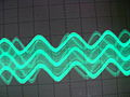
Imagine the following repeating waveform:

The green line is the waveform, the reddish vertical partial line represents the location of the trigger, and the yellow line represents the trigger level. If the scope was only fix to trigger on every rising border, this waveform would cause iii triggers for each bike:

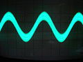
Bold the signal is fairly high frequency, the scope would probably look something like this:

On an bodily scope, each trigger would exist the aforementioned channel, so all would be the same color.

Information technology is desirable for the scope to simply trigger on one edge per cycle, so information technology is necessary to set the holdoff at slightly less than the period of the waveform. This prevents triggering from occurring more than once per bicycle, but still lets it trigger on the first edge of the adjacent bicycle.

Automatic sweep mode [edit]

Triggered sweeps tin can brandish a bare screen if in that location are no triggers. To avert this, these sweeps include a timing circuit that generates complimentary-running triggers and so a trace is ever visible. This is referred to as "auto sweep" or "automatic sweep" in the controls. Once triggers get in, the timer stops providing pseudo-triggers. The user volition unremarkably disable automatic sweep when observing low repetition rates.

Recurrent sweeps [edit]

If the input signal is periodic, the sweep repetition charge per unit can be adjusted to display a few cycles of the waveform. Early (tube) oscilloscopes and lowest-cost oscilloscopes take sweep oscillators that run continuously, and are uncalibrated. Such oscilloscopes are very simple, comparatively inexpensive, and were useful in radio servicing and some Tv servicing. Measuring voltage or time is possible, but simply with extra equipment, and is quite inconvenient. They are primarily qualitative instruments.

They have a few (widely spaced) frequency ranges, and relatively wide-range continuous frequency control within a given range. In use, the sweep frequency is ready to slightly lower than some submultiple of the input frequency, to display typically at least two cycles of the input signal (and then all details are visible). A very simple command feeds an adjustable amount of the vertical signal (or mayhap, a related external point) to the sweep oscillator. The signal triggers beam blanking and a sweep retrace sooner than it would occur free-running, and the display becomes stable.

Unmarried sweeps [edit]

Some oscilloscopes offer these. The user manually artillery the sweep excursion (typically by a pushbutton or equivalent). "Armed" ways it'southward ready to respond to a trigger. Once the sweep completes, it resets, and does non sweep once more until re-armed. This mode, combined with an oscilloscope camera, captures single-shot events.

Types of trigger include:

external trigger, a pulse from an external source continued to a dedicated input on the telescopic.
edge trigger, an edge detector that generates a pulse when the input indicate crosses a specified threshold voltage in a specified direction. These are the about common types of triggers; the level control sets the threshold voltage, and the slope command selects the direction (negative or positive-going). (The starting time sentence of the description as well applies to the inputs to some digital logic circuits; those inputs have fixed threshold and polarity response.)
video trigger, a circuit that extracts synchronizing pulses from video formats such every bit PAL and NTSC and triggers the timebase on every line, a specified line, every field, or every frame. This circuit is typically found in a waveform monitor device, though some meliorate oscilloscopes include this function.
delayed trigger, which waits a specified fourth dimension after an edge trigger before starting the sweep. As described under delayed sweeps, a trigger delay circuit (typically the main sweep) extends this delay to a known and adaptable interval. In this mode, the operator can examine a detail pulse in a long train of pulses.

Some recent designs of oscilloscopes include more sophisticated triggering schemes; these are described toward the terminate of this article.

Delayed sweeps [edit]

More sophisticated analog oscilloscopes incorporate a second timebase for a delayed sweep. A delayed sweep provides a very detailed wait at some small selected portion of the main timebase. The principal timebase serves as a controllable delay, after which the delayed timebase starts. This tin start when the delay expires, or tin can exist triggered (but) later the filibuster expires. Commonly, the delayed timebase is set for a faster sweep, sometimes much faster, such equally grand:ane. At extreme ratios, jitter in the delays on consecutive principal sweeps degrades the brandish, but delayed-sweep triggers tin can overcome this.

The display shows the vertical signal in one of several modes: the main timebase, or the delayed timebase only, or a combination thereof. When the delayed sweep is active, the main sweep trace brightens while the delayed sweep is advancing. In i combination style, provided only on some oscilloscopes, the trace changes from the master sweep to the delayed sweep once the delayed sweep starts, though less of the delayed fast sweep is visible for longer delays. Another combination mode multiplexes (alternates) the chief and delayed sweeps and then that both appear at once; a trace separation command displaces them. DSOs can display waveforms this way, without offering a delayed timebase as such.

Dual and multiple-trace oscilloscopes [edit]

Oscilloscopes with two vertical inputs, referred to equally dual-trace oscilloscopes, are extremely useful and commonplace. Using a single-axle CRT, they multiplex the inputs, usually switching between them fast enough to display two traces plainly at once. Less common are oscilloscopes with more traces; four inputs are common among these, but a few (Kikusui, for one) offered a display of the sweep trigger signal if desired. Some multi-trace oscilloscopes use the external trigger input as an optional vertical input, and some have third and fourth channels with only minimal controls. In all cases, the inputs, when independently displayed, are time-multiplexed, merely dual-trace oscilloscopes often can add together their inputs to brandish a existent-time analog sum. Inverting one channel while calculation them together results in a brandish of the differences between them, provided neither channel is overloaded. This difference mode tin provide a moderate-operation differential input.)

Switching channels tin can be asynchronous, i.eastward. free-running, with respect to the sweep frequency; or it tin can be done after each horizontal sweep is complete. Asynchronous switching is normally designated "Chopped", while sweep-synchronized is designated "Alt[ernate]". A given channel is alternately connected and asunder, leading to the term "chopped". Multi-trace oscilloscopes also switch channels either in chopped or alternate modes.

In general, chopped mode is better for slower sweeps. It is possible for the internal chopping rate to be a multiple of the sweep repetition rate, creating blanks in the traces, simply in practice this is rarely a problem. The gaps in one trace are overwritten past traces of the following sweep. A few oscilloscopes had a modulated chopping rate to avoid this occasional problem. Alternate mode, however, is ameliorate for faster sweeps.

True dual-beam CRT oscilloscopes did be, but were not mutual. I type (Cossor, U.G.) had a axle-splitter plate in its CRT, and single-ended deflection following the splitter. Others had ii complete electron guns, requiring tight control of axial (rotational) mechanical alignment in manufacturing the CRT. Beam-splitter types had horizontal deflection common to both vertical channels, just dual-gun oscilloscopes could have separate time bases, or utilise one time base for both channels. Multiple-gun CRTs (up to 10 guns) were made in past decades. With ten guns, the envelope (bulb) was cylindrical throughout its length. (Also encounter "CRT Invention" in Oscilloscope history.)

The vertical amplifier [edit]

In an analog oscilloscope, the vertical amplifier acquires the signal[s] to be displayed and provides a signal large enough to deflect the CRT's beam. In amend oscilloscopes, it delays the signal by a fraction of a microsecond. The maximum deflection is at least somewhat beyond the edges of the graticule, and more than typically some distance off-screen. The amplifier has to take depression baloney to brandish its input accurately (it must exist linear), and it has to recover speedily from overloads. As well, its time-domain response has to represent transients accurately—minimal overshoot, rounding, and tilt of a apartment pulse top.

A vertical input goes to a frequency-compensated pace attenuator to reduce large signals to prevent overload. The attenuator feeds one or more low-level stages, which in turn feed gain stages (and a filibuster-line driver if there is a delay). Subsequent gain stages lead to the final output phase, which develops a big signal swing (tens of volts, sometimes over 100 volts) for CRT electrostatic deflection.

In dual and multiple-trace oscilloscopes, an internal electronic switch selects the relatively low-level output of one aqueduct's early-stage amplifier and sends information technology to the post-obit stages of the vertical amplifier.

In free-running ("chopped") mode, the oscillator (which may exist but a different operating mode of the switch driver) blanks the beam before switching, and unblanks it only afterward the switching transients accept settled.

Part way through the amplifier is a feed to the sweep trigger circuits, for internal triggering from the point. This feed would be from an individual channel'south amplifier in a dual or multi-trace oscilloscope, the channel depending upon the setting of the trigger source selector.

This feed precedes the delay (if there is ane), which allows the sweep circuit to unblank the CRT and first the forwards sweep, so the CRT can show the triggering event. Loftier-quality analog delays add together a pocket-size cost to an oscilloscope, and are omitted in cost-sensitive oscilloscopes.

The filibuster, itself, comes from a special cablevision with a pair of conductors wound around a flexible, magnetically soft core. The coiling provides distributed inductance, while a conductive layer close to the wires provides distributed capacitance. The combination is a wideband manual line with considerable delay per unit length. Both ends of the delay cable require matched impedances to avoid reflections.

Ten-Y mode [edit]

Most modern oscilloscopes have several inputs for voltages, and thus can be used to plot one varying voltage versus some other. This is specially useful for graphing I-5 curves (electric current versus voltage characteristics) for components such as diodes, too as Lissajous patterns. Lissajous figures are an example of how an oscilloscope can be used to track phase differences between multiple input signals. This is very oftentimes used in broadcast applied science to plot the left and right stereophonic channels, to ensure that the stereo generator is calibrated properly. Historically, stable Lissajous figures were used to prove that two sine waves had a relatively uncomplicated frequency relationship, a numerically-small-scale ratio. They also indicated phase difference between 2 sine waves of the same frequency.

The 10-Y mode also lets the oscilloscope serve as a vector monitor to display images or user interfaces. Many early games, such equally Tennis for Ii, used an oscilloscope every bit an output device.^[12]

Complete loss of signal in an X-Y CRT brandish means that the axle is stationary, hitting a small spot. This risks burning the phosphor if the brightness is as well high. Such damage was more than common in older scopes every bit the phosphors previously used burned more hands. Some dedicated X-Y displays reduce beam current greatly, or bare the display entirely, if in that location are no inputs present.

Z input [edit]

Some analogue oscilloscopes feature a Z input. This is mostly an input terminal that connects straight to the CRT grid (usually via a coupling capacitor). This allows an external bespeak to either increase (if positive) or decrease (if negative) the brightness of the trace, even allowing it to be totally blanked. The voltage range to achieve cutting-off to a brightened brandish is of the order of 10–20 volts depending on the CRT characteristics.

An example of a practical awarding is if a pair of sine waves of known frequency are used to generate a circular Lissajous figure and a higher unknown frequency is applied to the Z input. This turns the continuous circle into a circumvolve of dots. The number of dots multiplied by the X-Y frequency gives the Z frequency. This technique simply works if the Z frequency is an integer ratio of the X-Y frequency and only if information technology is not so large that the dots become so numerous that they are difficult to count.

Bandwidth [edit]

Every bit with all practical instruments, oscilloscopes do non respond as to all possible input frequencies. The range of frequencies an oscilloscope can usefully display is referred to as its bandwidth. Bandwidth applies primarily to the Y-axis, though the X-axis sweeps must be fast enough to show the highest-frequency waveforms.

The bandwidth is defined as the frequency at which the sensitivity is 0.707 of the sensitivity at DC or the lowest Ac frequency (a drop of three dB).^[13] The oscilloscope'southward response drops off rapidly as the input frequency rises higher up that bespeak. Within the stated bandwidth the response is not necessarily exactly uniform (or "flat"), but should ever fall within a +0 to −3 dB range. I source^[thirteen] says there is a noticeable effect on the accuracy of voltage measurements at merely 20 percentage of the stated bandwidth. Some oscilloscopes' specifications exercise include a narrower tolerance range within the stated bandwidth.

Probes too have bandwidth limits and must be chosen and used to properly handle the frequencies of involvement. To achieve the flattest response, nearly probes must be "compensated" (an adjustment performed using a examination bespeak from the oscilloscope) to permit for the reactance of the probe's cable.

Some other related specification is ascent time. This is the elapsing of the fastest pulse that can exist resolved by the scope. It is related to the bandwidth approximately by:

Bandwidth in Hz ten ascent fourth dimension in seconds = 0.35.^[fourteen]

For example, an oscilloscope intended to resolve pulses with a ascension time of 1 nanosecond would have a bandwidth of 350 MHz.

In analog instruments, the bandwidth of the oscilloscope is express by the vertical amplifiers and the CRT or other display subsystem. In digital instruments, the sampling charge per unit of the analog-to-digital converter (ADC) is a factor, simply the stated analog bandwidth (and therefore the overall bandwidth of the instrument) is usually less than the ADC's Nyquist frequency. This is due to limitations in the analog betoken amplifier, deliberate design of the anti-aliasing filter that precedes the ADC, or both.

For a digital oscilloscope, a dominion of pollex is that the continuous sampling rate should be ten times the highest frequency desired to resolve; for example a twenty megasample/second rate would exist applicable for measuring signals upwardly to about 2 megahertz. This lets the anti-aliasing filter be designed with a iii dB down point of ii MHz and an effective cutoff at 10 MHz (the Nyquist frequency), avoiding the artifacts of a very steep ("brick-wall") filter.

A sampling oscilloscope tin display signals of considerably higher frequency than the sampling rate if the signals are exactly, or nearly, repetitive. It does this by taking one sample from each successive repetition of the input waveform, each sample being at an increased time interval from the trigger event. The waveform is then displayed from these collected samples. This mechanism is referred to as "equivalent-time sampling".^[xv] Some oscilloscopes tin can operate in either this style or in the more than traditional "existent-time" fashion at the operator's choice.

Other features [edit]

A computer model of the sweep of the oscilloscope

Some oscilloscopes accept cursors. These are lines that can be moved almost the screen to measure the time interval between two points, or the departure between 2 voltages. A few older oscilloscopes simply brightened the trace at movable locations. These cursors are more authentic than visual estimates referring to graticule lines.^[16] ^[17]

Amend quality full general purpose oscilloscopes include a calibration signal for setting up the bounty of test probes; this is (often) a i kHz foursquare-wave signal of a definite pinnacle-to-acme voltage available at a test concluding on the forepart panel. Some ameliorate oscilloscopes also have a squared-off loop for checking and adjusting electric current probes.

Sometimes a user wants to encounter an event that happens only occasionally. To catch these events, some oscilloscopes—chosen storage scopes—preserve the most recent sweep on the screen. This was originally achieved with a special CRT, a "storage tube", which retained the paradigm of even a very brief effect for a long time.

Some digital oscilloscopes can sweep at speeds equally slow as in one case per 60 minutes, emulating a strip chart recorder. That is, the signal scrolls beyond the screen from right to left. Most oscilloscopes with this facility switch from a sweep to a strip-chart way at nigh one sweep per x seconds. This is considering otherwise, the telescopic looks broken: information technology's collecting information, but the dot cannot be seen.

All but the simplest models of current oscilloscopes more often utilise digital signal sampling. Samples feed fast analog-to-digital converters, following which all signal processing (and storage) is digital.

Many oscilloscopes adapt plug-in modules for dissimilar purposes, e.g., high-sensitivity amplifiers of relatively narrow bandwidth, differential amplifiers, amplifiers with four or more channels, sampling plugins for repetitive signals of very loftier frequency, and special-purpose plugins, including audio/ultrasonic spectrum analyzers, and stable-offset-voltage direct-coupled channels with relatively high gain.

Examples of utilize [edit]

Lissajous figures on an oscilloscope, with xc degrees phase difference between x and y inputs

One of the near frequent uses of scopes is troubleshooting malfunctioning electronic equipment. For example, where a voltmeter may bear witness a totally unexpected voltage, a scope may reveal that the excursion is aquiver. In other cases the precise shape or timing of a pulse is important.

In a slice of electronic equipment, for instance, the connections between stages (e.g., electronic mixers, electronic oscillators, amplifiers) may exist 'probed' for the expected indicate, using the scope as a simple signal tracer. If the expected betoken is absent or incorrect, some preceding stage of the electronics is not operating correctly. Since most failures occur because of a single faulty component, each measurement tin can bear witness that some of the stages of a complex piece of equipment either work, or probably did not cause the fault.

In one case the faulty stage is found, further probing can ordinarily tell a skilled technician exactly which component has failed. Once the component is replaced, the unit of measurement can exist restored to service, or at least the adjacent fault can be isolated. This sort of troubleshooting is typical of radio and Television receivers, as well as sound amplifiers, but can apply to quite-dissimilar devices such equally electronic motor drives.

Another use is to bank check newly designed circuitry. Often, a newly designed excursion misbehaves because of pattern errors, bad voltage levels, electric dissonance etc. Digital electronics usually operate from a clock, and so a dual-trace scope showing both the clock signal and a test signal dependent upon the clock is useful. Storage scopes are helpful for "capturing" rare electronic events that cause defective operation.

Pictures of use [edit]

Heterodyne
Air-conditioning hum on sound
Sum of a low-frequency and a high-frequency bespeak
Bad filter on sine
Dual trace, showing dissimilar time bases on each trace

Automotive use [edit]

Get-go appearing in the 1970s for ignition system analysis, automotive oscilloscopes are becoming an important workshop tool for testing sensors and output signals on electronic engine management systems, braking and stability systems. Some oscilloscopes tin trigger and decode serial autobus messages, such every bit the CAN bus commonly used in automotive applications.

Choice [edit]

For piece of work at high frequencies and with fast digital signals, the bandwidth of the vertical amplifiers and sampling rate must be loftier enough. For general-purpose use, a bandwidth of at least 100 MHz is usually satisfactory. A much lower bandwidth is sufficient for audio-frequency applications but. A useful sweep range is from 1 second to 100 nanoseconds, with appropriate triggering and (for analog instruments) sweep delay. A well-designed, stable trigger circuit is required for a steady brandish. The chief benefit of a quality oscilloscope is the quality of the trigger excursion.^{[ citation needed ]}

Central choice criteria of a DSO (autonomously from input bandwidth) are the sample memory depth and sample rate. Early DSOs in the mid- to tardily 1990s but had a few KB of sample retentivity per aqueduct. This is adequate for bones waveform display, but does not permit detailed examination of the waveform or inspection of long data packets for example. Even entry-level (<$500) modernistic DSOs now have 1 MB or more of sample memory per channel, and this has become the expected minimum in any modernistic DSO.^{[ commendation needed ]} Often this sample retention is shared betwixt channels, and tin sometimes just be fully available at lower sample rates. At the highest sample rates, the retention may be express to a few tens of KB.^[eighteen] Any modern "real-fourth dimension" sample rate DSO typically has 5–10 times the input bandwidth in sample charge per unit. And so a 100 MHz bandwidth DSO would have 500 Ms/southward – 1 Gs/s sample rate. The theoretical minimum sample rate required, using SinX/ten interpolation, is 2.five times the bandwidth.^[nineteen]

Analog oscilloscopes have been almost totally displaced past digital storage scopes except for use exclusively at lower frequencies. Profoundly increased sample rates have largely eliminated the brandish of incorrect signals, known equally "aliasing", which was sometimes present in the first generation of digital scopes. The problem tin nevertheless occur when, for case, viewing a short section of a repetitive waveform that repeats at intervals thousands of times longer than the section viewed (for example a short synchronization pulse at the beginning of a particular idiot box line), with an oscilloscope that cannot shop the extremely big number of samples between one instance of the short department and the next.

The used test equipment market, especially on-line auction venues, typically has a wide option of older analog scopes available. Nevertheless it is condign more difficult to obtain replacement parts for these instruments, and repair services are generally unavailable from the original manufacturer. Used instruments are usually out of scale, and recalibration past companies with the equipment and expertise usually costs more the second-manus value of the instrument.^{[ citation needed ]}

Equally of 2007^[update], a 350 MHz bandwidth (BW), ii.5 gigasamples per second (GS/southward), dual-aqueduct digital storage telescopic costs about US$7000 new.^{[ commendation needed ]}

On the lowest end, an inexpensive hobby-form single-channel DSO could be purchased for nether $90 every bit of June 2011. These often accept limited bandwidth and other facilities, simply fulfill the basic functions of an oscilloscope.

Software [edit]

Many oscilloscopes today provide one or more than external interfaces to let remote musical instrument command by external software. These interfaces (or buses) include GPIB, Ethernet, serial port, USB and Wi-Fi.

Types and models [edit]

The following section is a brief summary of various types and models available. For a detailed discussion, refer to the other article.

Cathode-ray oscilloscope (CRO) [edit]

Example of an analog oscilloscope Lissajous figure, showing a harmonic human relationship of 1 horizontal oscillation cycle to 3 vertical oscillation cycles

The primeval and simplest type of oscilloscope consisted of a cathode ray tube, a vertical amplifier, a timebase, a horizontal amplifier and a power supply. These are now chosen "analog" scopes to distinguish them from the "digital" scopes that became common in the 1990s and later.

Analog scopes exercise not necessarily include a calibrated reference grid for size measurement of waves, and they may not display waves in the traditional sense of a line segment sweeping from left to right. Instead, they could be used for signal assay by feeding a reference signal into one axis and the signal to measure into the other axis. For an oscillating reference and measurement signal, this results in a circuitous looping pattern referred to as a Lissajous bend. The shape of the curve tin be interpreted to identify backdrop of the measurement signal in relation to the reference point, and is useful across a wide range of oscillation frequencies.

Dual-beam oscilloscope [edit]

The dual-axle analog oscilloscope can display two signals simultaneously. A special dual-beam CRT generates and deflects two separate beams. Multi-trace analog oscilloscopes can simulate a dual-beam brandish with chop and alternating sweeps—but those features do not provide simultaneous displays. (Existent time digital oscilloscopes offer the same benefits of a dual-beam oscilloscope, just they do non require a dual-beam display.) The disadvantages of the dual trace oscilloscope are that it cannot switch quickly betwixt traces, and cannot capture 2 fast transient events. A dual beam oscilloscope avoids those problems.

Analog storage oscilloscope [edit]

Trace storage is an extra feature available on some analog scopes; they used direct-view storage CRTs. Storage allows a trace pattern that normally would decay in a fraction of a second to remain on the screen for several minutes or longer. An electric circuit can then exist deliberately activated to store and erase the trace on the screen.

Digital oscilloscopes [edit]

While analog devices use continually varying voltages, digital devices use numbers that correspond to samples of the voltage. In the case of digital oscilloscopes, an analog-to-digital converter (ADC) changes the measured voltages into digital data.

The digital storage oscilloscope, or DSO for brusk, is the standard type of oscilloscope today for the majority of industrial applications, and thank you to the low costs of entry-level oscilloscopes fifty-fifty for hobbyists. Information technology replaces the electrostatic storage method in analog storage scopes with digital retention, which stores sample data as long as required without degradation and displays it without the brightness issues of storage-type CRTs. It likewise allows complex processing of the signal by high-speed digital indicate processing circuits.^[iii]

A standard DSO is limited to capturing signals with a bandwidth of less than half the sampling charge per unit of the ADC (called the Nyquist limit). There is a variation of the DSO called the digital sampling oscilloscope which tin exceed this limit for certain types of point, such as loftier-speed communications signals, where the waveform consists of repeating pulses. This type of DSO deliberately samples at a much lower frequency than the Nyquist limit so uses signal processing to reconstruct a composite view of a typical pulse.^[20]

Mixed-point oscilloscopes [edit]

A mixed-indicate oscilloscope (or MSO) has two kinds of inputs, a small number of analog channels (typically ii or four), and a larger number of digital channels (typically xvi). It provides the power to accurately fourth dimension-correlate analog and digital channels, thus offering a singled-out advantage over a carve up oscilloscope and logic analyser. Typically, digital channels may be grouped and displayed as a passenger vehicle with each bus value displayed at the bottom of the brandish in hex or binary. On most MSOs, the trigger can be set across both analog and digital channels.

Mixed-domain oscilloscopes [edit]

A mixed-domain oscilloscope (MDO) is an oscilloscope that comes with an additional RF input which is solely used for dedicated FFT-based spectrum analyzer functionality. Often, this RF input offers a higher bandwidth than the conventional analog input channels. This is in contrast to the FFT functionality of conventional digital oscilloscopes which utilise the normal analog inputs. Some MDOs allow fourth dimension-correlation of events in the fourth dimension domain (like a specific series information packet) with events happening in the frequency domain (like RF transmissions).

Handheld oscilloscopes [edit]

Handheld oscilloscopes are useful for many test and field service applications. Today, a hand held oscilloscope is usually a digital sampling oscilloscope, using a liquid crystal display.

Many paw-held and bench oscilloscopes accept the basis reference voltage common to all input channels. If more than than one measurement channel is used at the same fourth dimension, all the input signals must have the aforementioned voltage reference, and the shared default reference is the "earth". If there is no differential preamplifier or external signal isolator, this traditional desktop oscilloscope is not suitable for floating measurements. (Occasionally an oscilloscope user breaks the ground pin in the power supply cord of a bench-peak oscilloscope in an attempt to isolate the indicate common from the globe ground. This practise is unreliable since the entire stray capacitance of the musical instrument cabinet connects into the excursion. It is also a hazard to suspension a safety ground connection, and instruction manuals strongly advise against it.)

Some models of oscilloscope accept isolated inputs, where the signal reference level terminals are not connected together. Each input channel tin can be used to make a "floating" measurement with an independent bespeak reference level. Measurements can be made without tying one side of the oscilloscope input to the excursion signal mutual or ground reference.

The isolation available is categorized every bit shown beneath:

Overvoltage category	Operating voltage (effective value of Air-conditioning/DC to footing)	Peak instantaneous voltage (repeated twenty times)	Test resistor
CAT I	600 V	2500 V	30 Ω
CAT I	1000 V	4000 V	xxx Ω
CAT II	600 5	4000 V	12 Ω
Cat 2	1000 V	6000 V	12 Ω
True cat III	600 V	6000 V	2 Ω

PC-based oscilloscopes [edit]

PicoScope 6000 digital PC-based oscilloscope using a laptop computer for display & processing

Some digital oscilloscope rely on a PC platform for brandish and control of the instrument. This can exist in the grade of a standalone oscilloscope with internal PC platform (PC mainboard), or as external oscilloscope which connects through USB or LAN to a separate PC or laptop.

[edit]

A large number of instruments used in a variety of technical fields are really oscilloscopes with inputs, calibration, controls, display calibration, etc., specialized and optimized for a detail awarding. Examples of such oscilloscope-based instruments include waveform monitors for analyzing video levels in tv productions and medical devices such equally vital office monitors and electrocardiogram and electroencephalogram instruments. In automobile repair, an ignition analyzer is used to bear witness the spark waveforms for each cylinder. All of these are essentially oscilloscopes, performing the basic task of showing the changes in one or more input signals over time in an X‑Y brandish.

Other instruments convert the results of their measurements to a repetitive electrical bespeak, and incorporate an oscilloscope as a display element. Such complex measurement systems include spectrum analyzers, transistor analyzers, and fourth dimension domain reflectometers (TDRs). Dissimilar an oscilloscope, these instruments automatically generate stimulus or sweep a measurement parameter.

Come across also [edit]

Heart pattern
Phonodeik
Tennis for Ii, an oscilloscope game
Time-domain reflectometry
Vectorscope
Waveform monitor

References [edit]

^ How the Cathode Ray Oscillograph Is Used in Radio Servicing Archived 2013-05-24 at the Wayback Machine, National Radio Establish (1943)
^ "Cathode-Ray Oscillograph 274A Equipment DuMont Labs, Allen B" (in High german). Radiomuseum.org. Archived from the original on 2014-02-03. Retrieved 2014-03-fifteen .
^ ^a ^b ^c ^d Kularatna, Nihal (2003), "Fundamentals of Oscilloscopes", Digital and Analogue Instrumentation: Testing and Measurement, Institution of Engineering and Technology, pp. 165–208, ISBN978-0-85296-999-1
^ Marton, 50. (1980). "Ferdinand Braun: Forgotten Forefather". In Suesskind, Charles (ed.). Advances in electronics and electron physics. Vol. 50. Academic Press. p. 252. ISBN978-0-12-014650-five. Archived from the original on 2014-05-03. occurs start in a pair of afterwards papers past Zenneck (1899a,b)
^ The xx picofarad value is typical for telescopic bandwidths around 100 MHz; for example, a 200 MHz Tektronix 7A26 input impedance is 1M and 22 pF. (Tektronix (1983, p. 271); see also Tektronix (1998, p. 503), "typical loftier Z 10X passive probe model".) Lower bandwidth scopes used college capacitances; the 1 MHz Tektronix 7A22 input impedance is 1M and 47 pF. (Tektronix 1983, pp. 272–273) Higher bandwidth scopes utilise smaller capacitances. The 500 MHz Tektronix TDS510A input impedance is 1M and 10 pF. (Tektronix 1998, p. 78)
^ Probes are designed for a specific input impedance. They take compensation adjustments with a limited range, so they often cannot be used on different input impedances.
^ Wedlock & Roberge (1969)
^ Kobbe & Polits (1959)
^ Tektronix (1983, p. 426); Tek claims 300 MHz resistive coax at thirty pF per meter; schematic has 5 adjustments.
^ Zeidlhack & White (1970)
^ Jones, David. "Oscilloscope Trigger Holdoff Tutorial". EEVblog. Archived from the original on 28 January 2013. Retrieved 30 December 2012.
^ Nosowitz, Dan (2008-xi-08). "'Lawn tennis for Two', the Earth'south First Graphical Videogame". Retromodo. Gizmodo. Archived from the original on 2008-12-07. Retrieved 2008-xi-09 .
^ ^a ^b Webster, John G. (1999). The Measurement, Instrumentation and Sensors Handbook (illustrated ed.). Springer. pp. 37–24. ISBN978-3540648307.
^ Spitzer, Frank; Howarth, Barry (1972), Principles of modern Instrumentation , New York: Holt, Rinehart and Winston, p. 119 , ISBN0-03-080208-3
^ "Archived copy" (PDF). Archived (PDF) from the original on 2015-04-02. Retrieved 2015-03-20 . {{cite web}}: CS1 maint: archived re-create as title (link)
^ Hickman, Ian (2001). Oscilloscopes. Newnes. pp. 4, 20. ISBN0-7506-4757-iv . Retrieved 2022-01-15 .
^ Herres, David (2020). Oscilloscopes: A Manual for Students, Engineers, and Scientists. Springer Science+Business Media. pp. 120–121. doi:10.1007/978-three-030-53885-9. ISBN978-three-030-53885-9.
^ Jones, David. "DSO Tutorial". EEVblog. Archived from the original on 28 January 2013. Retrieved thirty December 2012.
^ "Minimum Required Sample Rate for a 1-GHz Bandwidth Oscilloscope" (PDF). keysight.com. Keysight Technologies. Archived (PDF) from the original on 16 June 2013. Retrieved thirty December 2012.
^ Green, Leslie (June 21, 2001), "The alias theorems: applied undersampling for expert engineers", EDN, archived from the original on xx June 2013, retrieved 11 October 2012

Usa 2883619, Kobbe, John R. & Polits, William J., "Electric Probe", published 1959-04-21
Tektronix (1983), Tek Products, Tektronix
Tektronix (1998), Measurement Products Catalog 1998/1999, Tektronix
Matrimony, Bruce D.; Roberge, James M. (1969), Electronic Components and Measurements, Prentice-Hall, pp. 150–152, Bibcode:1969ecm..book.....W, ISBN0-xiii-250464-two
U.s. 3532982, Zeidlhack, Donald F. & White, Richard Yard., "Transmission Line Termination Circuit", published 1970-ten-06

External links [edit]

The Cathode Ray Tube site
Virtual Oscilloscope Museum
An interactive online oscilloscope demonstration

Source: https://en.wikipedia.org/wiki/Oscilloscope

Posted by: mccrayearre1983.blogspot.com